The following Julia programme implements the so-called FastShift algorithm for fast matrix multiplication of integer matrices using bit operations and recursive subdivision. Comments in the source code explain important parts of the implementation.
# 🔠 FastShift Algorithm in Julia, Authors: Boris Haase & Math AI 🧠 from April 17, 2025
using LinearAlgebra, BenchmarkTools, Printf, Random, Base.Threads
const D = 256                                        # Ceiling value, less than or equal to G
const E = 8                                          # Exponent roughly greater than five
const R = 64                                         # Threshold for switching to multithreading
const G = 1  << E                                    # Desired upper bit limit
const I = BigInt(1)                                  # One  as a BigInt
const L = (I << D) - I                               # Upper/lower limit for random values
const T = AbstractMatrix{BigInt}                     # Matrix type for large integers
const S = G  << 1                                    # Shift factor as a power of two
const O = BigInt(0)                                  # Zero as a BigInt

# 🔧 Helper functions for modular division and matrix multiplication
remR(x, t, u, v) =  x < O ? -adjR(-x & u, t, v) : adjR(x & u, t, v)
adjR(x, t, v)    =  x < v ? x : x - t
divR(x, v, s)    = (x + v) >> s

function simd_mul(A::T, B::T, n::Int)::T             # Conventional SIMD matrix multiplication
    C = zeros(BigInt, n, n)
    @inbounds for i in 1:n                           # No bounds checking for indices
        for j in 1:n
            z = O
            @simd ivdep for k in 1:n                 # No interdependencies in this loop
                z += A[i, k] * B[k, j]
            end
            C[i, j] = z
        end
    end
    return C                                         # Return the matrix product
end

# 🔡 FastShift recursive multiplication for matrices of large integers
function fastshift(A::T, B::T, n::Int, s::Int)::T
    n <= R && return simd_mul(A, B, n)               # Use standard multiplication for small n

    m = n >> 1                                       # Split matrices into four blocks
    M =    1:m                                       # Left  index of the matrix
    N =  m+1:n                                       # Right index of the matrix
    v = I << (s - 1)                                 # Reference value for nearest neighbour
    t = I << s                                       # Modulus for division with remainder
    r = s << 1                                       # Next recursion depth
    u = t -  I                                       # Bitmask to extract the lower half

    R1 = (B[M, M] .<< s) .+ B[M, N]                  # Top    row of combined matrix
    R2 = (B[N, M] .<< s) .+ B[N, N]                  # Bottom row of combined matrix

    if n > R                                         # Use threads for large matrices
        t1 =  @spawn fastshift(A[M, M], R1, m, r)
        t2 =  @spawn fastshift(A[M, N], R2, m, r)
        t3 =  @spawn fastshift(A[N, M], R1, m, r)
        S4 =         fastshift(A[N, N], R2, m, r)    # Matrix on main thread
        S1 =  fetch(t1)                              # Retrieve results from other threads
        S2 =  fetch(t2)
        S3 =  fetch(t3)
    else
        S1 =         fastshift(A[M, M], R1, m, r)    # No threading for small matrices
        S2 =         fastshift(A[M, N], R2, m, r)
        S3 =         fastshift(A[N, M], R1, m, r)
        S4 =         fastshift(A[N, N], R2, m, r)
    end

    C1 = divR.(S1, v, s   ) .+ divR.(S2, v, s   )    # Modular division as defined
    C2 = remR.(S1, t, u, v) .+ remR.(S2, t, u, v)
    C3 = divR.(S3, v, s   ) .+ divR.(S4, v, s   )
    C4 = remR.(S3, t, u, v) .+ remR.(S4, t, u, v)

    return [C1 C2; C3 C4]                            # Return the full matrix product
end

# 🕔 Benchmark for C = A * B with correctness check against Julia's standard implementation
function main()
    @assert D <= G "Ceiling value must not exceed bit limit G"
    println("⏱️ Benchmark for the FastShift algorithm – m from 1 to 10")
    println("═════════════════════════════════════════════════════════")
    println("🕸 Threads: $(nthreads())")             # Expected to run with four threads

    for m in 1:10
        n  = 1 << m                                  # Dimension as a power of two
        A  = rand(-L:L, n, n)                        # Left  random matrix with large integers
        B  = rand(-L:L, n, n)                        # Right random matrix with large integers

        println("\n❓ Test: 2^$m × 2^$m → $n × $n")  # Display test info
        t_fasts = @elapsed C_fasts = fastshift(A, B, n, S + m)
        @printf("🔢 Runtime for FastShift: %10.4f seconds\n", t_fasts)

        t_julia = @elapsed C_julia = A * B           # Measure Julia's standard multiplication
        @printf("❕ Runtime for Julia A*B: %10.4f seconds\n", t_julia)
        println("💯 Equality of results:")           # Check if results match
        println(C_fasts == C_julia ? "✅ FastShift ≙ Julia" : "❌ FastShift ≠ Julia")
    end
end

# ▶️ Start execution
main()
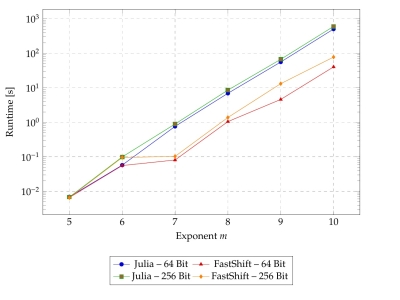
| \(m\) | \(T_j^{64}\) | \(T_f^{64}\) | \(T_j^{64}\)/\(T_f^{64}\) | \(T_j^{256}\) | \(T_f^{256}\) | \(T_j^{256}/T_f^{256}\) |
|---|---|---|---|---|---|---|
| 5 | 0.0069 | 0.0066 | 1.0455 | 0.0068 | 0.0065 | 1.0462 |
| 6 | 0.0573 | 0.0557 | 1.0287 | 0.0988 | 0.0951 | 1.0389 |
| 7 | 0.7557 | 0.0805 | 9.3882 | 0.8866 | 0.1026 | 8.6414 |
| 8 | 6.8593 | 1.0416 | 6.5865 | 8.4964 | 1.3699 | 6.2029 |
| 9 | 55.2878 | 4.5610 | 12.1228 | 66.0994 | 13.0518 | 5.0654 |
| 10 | 496.9587 | 39.9252 | 12.4443 | 592.4100 | 76.8205 | 7.7094 |
Modeling the Runtime Behaviour
The runtime can be further reduced by using suitable pointer arithmetic. The nonlinear function \(T_n \sim n^a\) modeled with Mathematica and compared with both \(T_n \sim n^{\hat{a}}\) and \(T_n \sim n^{\hat{a}} + b\) yields the following results for 64 bit: \(T_j^{64} = \mathcal{O}(n^{2.32})\) and \(T_f^{64} = \mathcal{O}(n^{1.96})\). Analogously, 256 bit yields: \(T_j^{256} = \mathcal{O}(n^{2.35})\) and \(T_f^{256} = \mathcal{O}(n^{2.05})\).
© 2025 by Boris Haase