Youth researches 1983
Subject area physics
A novel method for the determination of the periodic time of the mathematical pendulum with large amplitudes and the discussion for the applicability on other selected oscillations of the plane
Compiled by Boris Haase (18),
Theodor-Heuss-Gymnasium in Göttingen
Abstract of the present paper
The oscillation period of mass points on curved oscillation ways in the vertical plane – like e.g. the mathematical pendulum and the cycloid pendulum -, is to be computed in the present paper in a simpler way than so far.
Most of these oscillation periods are – if the mass point on the oscillation way is far from the rest position, whose lowest point – dependent on this distance, which makes the computation generally more difficult.
In order to be able to compute an independent periodic time of this distance, the amplitude, we must know, except the mass, only the direction parameter, the quotient from repelling force and corresponding amplitude respectively direction way.
This knowledge is extended and applied in this paper to the oscillation period dependent on its amplitude.
Here partially differences to the conventional methods arise – by the example of the mathematical pendulum up to at most one per cent for 90° of amplitude – which is partially not the case as can be seen by the example of the cycloid pendulum, however. No references could be found for the ellipse pendulum, which has been also treated.
In the experimental part, the calculated periodic time could be confirmed for the mathematical pendulum considering the sources of error and the measuring accuracy.
The author concludes that the independently developed procedure could be well used in physics.
Table of contents
|
1. |
Introduction |
|
2. |
Main Part |
|
2.2. |
Experiment to the Mathematical Pendulum |
|
2.3. |
Calculations of Errors |
|
2.4. |
Discussion |
|
3. |
Conclusion |
|
4. |
Appendix |
|
5. |
Bibliography |
1. Introduction
1.1. Reason and Basic Idea
The periodic time of the mathematical pendulum for large amplitudes was determined so far by quite difficult procedures of the infinitesimal calculus and series expansion. The new procedure developed in the present paper to determine the periodic time for selected oscillations of the plane is to simplify the calculation method on the one hand, on the other hand it is to compare with the old procedure for two examples regarding its accuracy.
Basic idea is the simultaneous simulation of the respective pendulum oscillation by a straight-lined harmonic oscillation (spring pendulum, oscillator).
1.2. Presuppositions
All selected oscillations emanate from a mass point, which is to swing in the vertical plane at a thread without mass around a fix point. The pendulum thread may be pulled to the side here – viewed from the rest position – at most by 90°, since the maximally repelling force must lie at initial height, in which no additional acceleration is to arise.
In order to prevent a free fall, otherwise bars would have to be used instead of threads, which could not, however, (as necessary) be clung to evolutes of the oscillation ways. Despite the clinging, the length of the pendulum is assumed in rest position for simplification reasons.
The radius of curvature of the oscillation way must remain either constant from the rest position or be continuously reduced, so that a free fall is prevented, too.
Friction and damping aspects are to be neglected.
Otherwise further computations are necessary for the periodic time, which would go however beyond the scope of this paper.
2. Main Part
2.1. Theoretical Solution of the Problem
2.1.1. General Solution
The periodic time of a harmonic oscillation is given by:\[(a)\;T = 2\pi \sqrt {{\textstyle{m \over D}}}.\]After the principle of conservation of energy holds:\[(b)\;\tfrac{1}{2} m v^{2} = \tfrac{1}{2} D s^{2} = m g h.\]During an oscillation form the potential energy \(W_{pot}\) and the kinetic energy \(W_{kin}\) the constant sum:\[(c)\;W_{pot} + W_{kin} = W_{pot_{0}}.\]\(W_{pot_{0}}\) is to be expressed now by the tension energy \(W_{Sp}\), in order to determine a direction parameter \(D(\varphi_{0})\), dependent on the amplitude. \(D(\varphi_{0})\) is to be inserted then into the formula (a) for the determination of the periodic time.
For this purpose, an ersatz movement of the mass \(m\) is necessary by force \(F\) on the direction way \(s\). We have:\[(d)\;D = F/s \text{ (Hooke’s law) and}\]\[{\rm{(e)}}\;{\rm{F}}\, = \,{\rm{m}}\,{\rm{a}} = \,{\rm{m}}\,{\rm{l}}\,\ddot \varphi \,\,\left( {{\text{Newton}}} \right).\] Furthermore, we always resort to the direction parameter \(D\) of the plane thread pendulum for minimal amplitude. Here we have for the repelling and to the oscillation way tangential force \(F_{R}\), since the normal force is compensated by the tension force of the thread (1, 2):\[{\rm{(f)}}\;{{\rm{F}}_{\rm{R}}} = \,{\rm{m}}\,{\rm{g}}\,{\rm{sin}}\,\varphi = \, – m\,l\,\ddot \varphi .\]From this follows:\[(g)\;\ddot \varphi \, = \,\,{\rm{sin}}\,\varphi \,{\textstyle{g \over l}}.\]For smallest amplitude angles \(\varphi \; sin(\varphi)\) can be replaced by \(\varphi\), and the conditions apply to the harmonic oscillation. Therefore, we have:\[(h)\;\ddot \varphi \, = {\omega ^2}\,\varphi \]and from (g) follows:\[(i)\;\omega = \sqrt {{\textstyle{g \over l}}.} \]Thus, we have:\[(j)\;D = m\,{\omega ^2} = m\,{\textstyle{g \over l}}.\]For larger amplitudes the direction parameter \(D\) must consist of the product of the direction parameter for the harmonic oscillation in terms of a function value \(f(\varphi_{0})\) of the amplitude angle \(\varphi\) determining the inharmonic oscillation.
We write:\[(k)\;D({\varphi _0}) = \left( {m{\textstyle{g \over l}}} \right)\,f({\varphi _0}).\]The function value \(f(\varphi_{0})\), however, is not defined for the harmonic condition of the energy theorem, so that it must cancel if it is introduced. Writing \(s = x l\) we have:\[(l)\;\frac{1}{2}\frac{{\frac{{f({\varphi _0})mxg}}{{xl}}{{(xl)}^2}}}{{f({\varphi _0})}} = m\,g\,h.\]Hereby the not changing direction way \(s\) can be computed by the energy theorem, if one assigns the function value \(f(\varphi_{0})\) to the repelling force \(F_{R}\). Writing\[{\textstyle{1 \over 2}}\left( {m{\textstyle{g \over l}}} \right){s^2} = m\,g\,h\]we have for the direction way:\[(m)\;s = \sqrt {2lh} .\]The repelling force \(F_{R}\) must be developed thus independently from the energy theorem. It is rather fixed by the initial oscillation as the tangentially attacking and thus maximally repelling force at initial height of the oscillation way. From\[(n)\;F_{R} = (-) m a,\]we obtain the periodic time with (a) and (d):\[(o)\;T = 2\pi \sqrt {\frac{{\sqrt {2lh} }}{a}} .\] Vividly, the direction way \(s\) represents with (m) the chord of a circle with the radius l. Since this circle is circle of curvature for the rest position of the oscillation way, this chord must lead from one point of the circular path at the initial height \(h\) to the rest position.
The mathematical pendulum (fig. 1) is the simplest form of an oscillation way, which aligns with the circle of curvature and possesses a punctiform evolute. Therefore, this is to be treated first.
2.1.2. The Mathematical Pendulum
From fig. 1, we obtain for the direction way \(s\):\[s = 2\sin \left( {{\textstyle{{{\varphi _0}} \over 2}}} \right)l.\] With respect to (f), we have for the maximally repelling force \(F_{R}\):\[F_{R} = (-) m g\, \text{sin}(\varphi_{0}).\]The periodic time is regarding (a) and (d) therefore:\[T = 2\pi \sqrt {\frac{l}{{\cos \left( {{\textstyle{{{\varphi _0}} \over 2}}} \right)g}}.} \]
2.1.3. The Cycloid Pendulum
The common cycloid (fig. 2) has the parameter equation (2):\[x = a (\Phi – \text{sin}(\Phi)) \text{ and } y = a (\text{cos}(\Phi) – 1).\] We obtain for the radius of curvature \(\rho\):\[\rho = 4a\sin \left( {{\textstyle{\phi \over 2}}} \right).\]Since the angles \(\Phi\) increase from the initial height \(h\) to the rest position with \(\Phi = \pi\) or the sine decreases from \(\Phi/2\) after exceeding the rest position towards the reversal point, the qualifications for the computation of the periodic time are fulfilled.
The initial height is:\[h = 2 a + y = a (\text{cos}(\Phi_{0}) + 1).\]If we plug \(h\) in (m), we have for \(l = 4 a\):\[s = l\sqrt {{\textstyle{{\cos \,{\phi _0} + 1} \over 2}}} = \cos \left( {{\textstyle{{{\phi _0}} \over 2}}} \right)l.\]Since the tangential acceleration \(b_{t}\) works always vertically to the radius of curvature \(\rho\), we obtain:\[{b_t} = \alpha \cos \left( {{\textstyle{{{\phi _0}} \over 2}}} \right)g.\]If \(\Phi_{0} = 0\), then \(b_{t} = g\), if \(\Phi_{0} = \pi\), then \(b_{t} = 0\). Therefore the multiplier \(\alpha = 1\) and we have:\[{b_t} = \cos \left( {{\textstyle{{{\phi _0}} \over 2}}} \right)g.\]With respect to (o), the periodic time finally is:\[T = 2\pi \sqrt {{\textstyle{l \over g}}} .\]This was already proven by Huygens centuries ago.
2.1.4. The Ellipse Pendulum
The ellipse (fig. 3) has the parameter equation (3):\[\frac{{{x^2}}}{{{a^2}}} + \frac{{{y^2}}}{{{b^2}}} = 1.\] By differentiating the radius of curvature \(\rho\) we obtain (see appendix):\[\rho = \frac{{\left({{{a^4} – {a^2}{x^2} + {b^2}{x^2}}}\right)}^{\tfrac{3}{2}}}{{{a^4}b}}.\]From the rest position, where \(x = 0\), \(x\) increases towards the reversal points, and since \(a^{2} x^{2} > b^{2} x^{2}\) holds, the radius of curvature is continuously reduced. We obtain thus for the rest position \(\rho\):\[\rho = l = \frac{{{a^2}}}{b}.\]Writing\[y = – b\sqrt {1 – \frac{{{x^2}}}{{{a^2}}}} \]the initial height \(h\) is:\[h = b + y = b\left( {1 – \sqrt {1 – \frac{{{x^2}}}{{{a^2}}}} } \right).\]Applying (m) we have thus for the direction way \(s\):\[s = \sqrt {2a\left( {a – \sqrt {{a^2} – {x^2}} } \right)} .\]Hence, the direction way is independent of the semi-minor axis of the ellipse.
The tangential acceleration \(b_{t}\) is (after fig. 3):\[{b_t} = \cos \,\beta \,g = \frac{{bxg}}{{\sqrt {{a^4} – {a^2}{x^2} + {b^2}{x^2}} }}.\]Applying (o) we obtain for the periodic time:\[T = 2\pi \sqrt {\frac{{\sqrt {{a^4} – {a^2}{x^2} + {b^2}{x^2}} \sqrt {2a\left( {a – \sqrt {{a^2} – {x^2}} } \right)} }}{{bxg}}} .\]Although the periodic time is not defined for \(x = 0\), we have for very small \(x\), however:\[T = 2\pi \sqrt {\frac{{{a^2}}}{{bg}}} = 2\pi \sqrt {\frac{l}{g}} .\]For \(x = a\), the proposition follows:
The periodic time on an ellipse with maximum amplitude is independent of the semi-minor axis.
2.2. Experiment to the Mathematical Pendulum
The experimental part was limited to the mathematical pendulum for temporal reasons.
Not only crafting evolutes would be otherwise very effortful, but also larger sources of error would be opened during the cycloid or ellipse oscillation. The difficulty to let the pendulum swing exactly to the evolute is an example for that, since the pendulum leaves the vertical plane already after few oscillations. Moreover, impulse or friction forces arise with the beginning of the swinging and in the bearing, which let the respective pendulum become the mathematical pendulum for large amplitudes.
The latter can be regarded therefore as part for the whole.
2.2.1. Experimental Setup
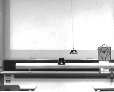
Two bars of a meter are connected to a third one and four sleeves and are pushed symmetrically through two ceiling hooks. In the centre, we fix additionally a protractor and the bearing for the pendulum thread of 1.60 m length.
An air track is placed in parallel to it on the bench such that its centre is vertically under the point of the protractor. A car of 0.2 kg mass placed on the centre is clamped by two springs such that we obtain a direction parameter of 2 N/m between the clamping at the end of the bench and the car.
A stopwatch is mounted ready to hand regarding the initial height of the pendulum and the car.
The experiment is illustrated at the beginning. All devices used are specified also in the appendix.
2.2.2. Test Procedure and Results
First, we assured ourselves of the independence of the periodic time of the mass of the pendulum by attaching once a approx. 5 kg heavy ball, another time the car weighted on 1 kg of mass to the pendulum thread. The difference of the measured periodic time amounted to hundredths a second on each of the ten periods.
During the simulation of the mathematical pendulum by the harmonic oscillator, the time difference per oscillation amounted to 0.6 s (back and forth) with ten oscillations and 60° of maximum amplitude of the pendulum.
Computing the mass of the harmonic oscillator we used the formula:\[m = \frac{{2lD}}{{\cos \left( {{\textstyle{{{\varphi _0}} \over 2}}} \right)g}}.\]The latter can be determined directly from the periodic times for the two systems.
Here the direction parameter \(D_{0}\) for the oscillator is twice as much the equal spring constants of the used tension springs. The periodic time of the oscillator is therefore:\[T = 2\pi \sqrt {\frac{m}{{2D}}} \,(4).\]The periodic time of the mathematical pendulum calculated above is:\[T = 2\pi \sqrt {\frac{l}{{\cos \left( {{\textstyle{{{\varphi _0}} \over 2}}} \right)g}}} .\]The damping of the pendulum for amplitude 60° amounted to 1°, whereas the oscillator had one of 0.01 m for amplitude 0.9 m.
The appendix specifies the measured values for amplitudes of the mathematical pendulum from 0° to 90° in tab. 1.
2.3. Computations of errors
The periodic time of the mathematical pendulum was so far specified via the elliptical integral\[\int\limits_0^{{\textstyle{\pi \over 2}}} {\frac{{d\phi }}{{\sqrt {1 – {k^2}{{\sin }^2}\phi } }}} \,\]where\[\,k = \sin \left( {{\textstyle{{{\varphi _0}} \over 2}}} \right)\,\]giving (2):\[T = 2\pi \sqrt {{\textstyle{l \over g}}\left( {1 + {{\left( {{\textstyle{1 \over 2}}} \right)}^2}{k^2} + {{\left( {{\textstyle{{1 \cdot 3} \over {2 \cdot 4}}}} \right)}^2}{k^4} + {{\left( {{\textstyle{{1 \cdot 3 \cdot 5} \over {2 \cdot 4 \cdot 6}}}} \right)}^2}{k^6} + …} \right)} .\]To make a direct comparison with the new formula for the periodic time:\[T = 2\pi \sqrt {\frac{l}{{\cos \left( {{\textstyle{{{\varphi _0}} \over 2}}} \right)g}}} .\]the function value\[f({\varphi _0}) = \sqrt {\frac{1}{{\cos \left( {{\textstyle{{{\varphi _0}} \over 2}}} \right)}}} \] is converted by means of the series where \(|x| < 1\):\[{(1 + x)^p} = 1 + px + \frac{{p(p – 1){x^2}}}{{1 \cdot 2}} + \frac{{p(p – 1)(p – 2){x^3}}}{{1 \cdot 2 \cdot 3}} + …\,\,(2)\]and the relationship:\[f({\varphi _0}) = \frac{1}{{\sqrt[{4}]{{1 – {{\sin }^2}\left( {{\textstyle{{{\varphi _0}} \over 2}}} \right)}}}}\] with respect to\[x = – {\sin ^2}\left( {{\textstyle{{{\varphi _0}} \over 2}}} \right) = – {k^2}\]into the comparison series:\[1 + {\left( {{\textstyle{k \over 2}}} \right)^2} + {\left( {{\textstyle{{1 \cdot 5} \over {1 \cdot 2}}}} \right)^2}{\left( {{\textstyle{k \over 2}}} \right)^4} + {\left( {{\textstyle{{1 \cdot 5 \cdot 9} \over {1 \cdot 2 \cdot 3}}}} \right)^2}{\left( {{\textstyle{k \over 2}}} \right)^6} + …\;.\]It follows that the two series are identical up to the first square member.
If we divide the old by the new series and subtract 1, we obtain the series of the relative error, where the former has a smaller modulus:\[{\textstyle{1 \over {64}}}{k^4} + {\textstyle{1 \over {64}}}{k^6} + {\textstyle{{231} \over {16384}}}{k^8} + …\,\,.\]If we divide conversely with identical subtraction, the relative error is larger:\[{\textstyle{1 \over {64}}}{k^4} + {\textstyle{1 \over {64}}}{k^6} + {\textstyle{{235} \over {16384}}}{k^8} + …\,\,.\]The number of the absolute error is the result of subtracting the old from the new series:\[{\textstyle{1 \over {64}}}{k^4} + {\textstyle{5 \over {256}}}{k^6} + {\textstyle{{335} \over {16384}}}{k^8} + …\,\,.\] The appendix records the values for selected angles from 0° to 90° of all series specified here in tables.
2.4. Discussion
Here the proportionalities arising from the formula are once to be considered:\[\,T = 2\pi \sqrt {\frac{{\sqrt {2lh} }}{a}}.\] First, it is to be noted that the direction way \(s\) is not proportional to the acceleration \(a\) of the repelling force \(F_{R}\), but we must consider the function value \(f(\varphi_{0})\), contained in \(a\).
The length of the oscillation way is adapted via the direction way:
If the initial height \(h\) is very small, the distance to be covered becomes smaller on the oscillation way in \(y\)-direction, and hence the periodic time, too.
If the oscillation way is moreover very flat, the small initial height is confronted by a large pendulum length, so that we obtain a mean for the length of the direction way, as it appears very clearly for maximum amplitudes of the ellipse pendulum.
For highly curved oscillation ways and large initial heights, the periodic time is relatively larger as with the mathematical pendulum.
In the direct proximity of the rest position, the numerical values of direction way and acceleration cancel out, so that the direction way becomes the length \(l\) of the pendulum and the acceleration becomes the standard acceleration \(g\).
In the rest position itself, the periodic time is strictly speaking not defined, because the initial height \(h\) and the acceleration \(a\) become zero there.
The larger the acceleration \(a\), the smaller the periodic time is, otherwise reverse conditions do exist.
These insights could be relative well confirmed in the experiment for the mathematical pendulum.
3. Conclusion
We can say in retrospect that the actual approach is not completely consistent with the one stated for clarity reasons.
Thus, first the problem of the mathematical pendulum was solved and then a general problem solution was established. All periodic times were computed without knowledge of the periodic times given in the corresponding literature, which was consulted several weeks later, when the experiment took place.
The calculation method could indeed be much simplified and the margin of error of 0.01 or one per cent needed not be exceeded regarding the accuracy for the old procedure.
Here the ellipse pendulum could not be included, since no references could be found about its periodic time.
The margin of error will most likely shift upwards, however, since the mathematical pendulum as special case of the ellipse pendulum such that its periodic time can be transferred for semi axes of equal length to the one of the mathematical pendulum, already deviates barely one per cent for maximum amplitude in relation to its periodic time.
The periodic time of the cycloid pendulum is, however, consistent with the references.
3.1. Critical Appreciation of the Paper
Without doubt, the problem of evolutes is not yet completely solved. If we do not presuppose anymore the pendulum length in rest position, we have perhaps again to resort to procedures of the infinitesimal calculus and series expansion, in order to obtain a higher precision.
On the one hand the mathematical pendulum, on the other hand the cycloid pendulum is contradictory to that.
For the first one, a distinct evolute is missing despite deviation, for the latter there is no deviation despite the presence of an evolute.
Thus, the new procedure must be considered as independent.
Measuring further periodic times than that of the mathematical pendulum is unfortunately missing in this paper and would clarify the circumstances more exactly. Here, however, very high requirements have to be put on the measuring accuracy and on the course of the experiments.
Altogether, the procedure developed in this paper requires a certain adjustment concerning the way of thinking; nevertheless, it should be applicable due to the good results obtained in physics.
4. Appendix
Figures
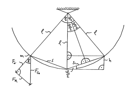
Fig. 1
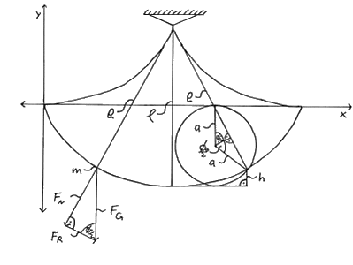
Fig. 2
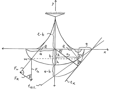
Fig. 3
All constructions took place with the aid of (9).
Auxiliary Calculations
The general formula (3) applies for the radius of curvature:\[\rho = \frac{{{{\left( {{{\dot x}^2} + {{\dot y}^2}} \right)}^{{\textstyle{3 \over 2}}}}}}{{\dot x\ddot y – \dot y\ddot x}}.\]The common cycloid has the parameter equation (2):\[x = a (\Phi – \text{sin}\,(\Phi)) \text{ and } y = a (\text{cos}(\Phi) – 1).\]For\[{\left( {{{\dot x}^2} + {{\dot y}^2}} \right)^{{\textstyle{3 \over 2}}}},\]we can write therefore \[{\left( {{a^2} – 2\cos \,\phi \,{a^2} + {{\cos }^2}\phi \,{a^2} + {{\sin }^2}\phi \,{a^2}} \right)^{{\textstyle{3 \over 2}}}} = {\left( {2{a^2} – 2\cos \phi \,{a^2}} \right)^{{\textstyle{3 \over 2}}}}.\]For\[\dot x\ddot y – \dot y\ddot x = (a – \cos \,\phi \,a)( – \cos \,\phi \,a) – ( – \sin \,\phi \,a)\sin \,\phi \,a = {a^2} – \cos \,\phi \,{a^2},\]we have thus for the radius of curvature\[\rho = 2a\sqrt {2(1 – \cos \,\phi )} = 4\,a\,\sin \left( {{\textstyle{\phi \over 2}}} \right).\]If we write for the ellipse temporarily \(x = \text{sin}\,(\varphi) a\) and\[y = – b\sqrt {1 – {\textstyle{{{x^2}} \over {{a^2}}}}} = – \cos \,\varphi \,\,b,\]we obtain:\[\dot x\ddot y – \dot y\ddot x = \cos \,\varphi \,\,a(\cos \,\varphi \,\,b) – \sin \,\varphi \,\,b( – \sin \,\varphi \,\,a) = ab.\]Thereby, the radius of curvature is:\[\rho = \frac{{{{\left( {{{\cos }^2}\varphi \,\,{a^2} + {{\sin }^2}\varphi \,\,{b^2}} \right)}^{{\textstyle{3 \over 2}}}}}}{{ab}}.\] If we revoke the transformation, we obtain for \(\rho\) after expanding the fraction by \(a^{3}\):\[\rho = \frac{{{{\left( {{a^4} – {a^2}{x^2} + {b^2}{x^2}} \right)}^{{\textstyle{3 \over 2}}}}}}{{{a^4}b}}.\]The evolute of the common cycloid is also a cycloid with identical \(a\) (5).
For the evolute of the ellipse, we have, however, by (6):\[\xi = \frac{{({a^2} – {b^2}){{\cos }^3}t}}{a}\]and\[\,\eta = \frac{{({a^2} – {b^2}){{\sin }^3}t}}{b}\]for \(x = a \text{ cos}(t)\) and \(y = b \text{ sin}\,(t)\).
The following initial considerations are necessary to compute the tangential acceleration \(b_{t}\) of the ellipse:\[\tan \gamma = \frac{{\sqrt {{a^2} – {x^2}} }}{x} = \frac{q}{{\sqrt {{a^2} – {x^2}} }}.\]From this follows directly:\[q = \frac{{{a^2} – {x^2}}}{x}.\]We can write for\[\cos \,\beta = \frac{y}{{\sqrt {{q^2} + {y^2}} }} = \frac{y}{{{{\sqrt {{{\left( {\frac{{{a^2} – {x^2}}}{x}} \right)}^2} + {y^2}} }^{}}}}\]after expanding by\[\frac{{ax}}{{\sqrt {{a^2} – {x^2}} }}\]\[\cos \,\beta = \frac{{bx}}{{\sqrt {{a^4} – {a^2}{x^2} + {b^2}{x^2}} }}.\]To convert the formula for the periodic time of the ellipse pendulum:\[T = 2\pi \sqrt {\frac{{\sqrt {{a^4} – {a^2}{x^2} + {b^2}{x^2}} \sqrt {2a\left( {a – \sqrt {{a^2} – {x^2}} } \right)} }}{{bxg}}} \]into that of the mathematical pendulum, let \(x = \text{sin}\,(\varphi_{0}) a\) and \(a = b = 1\). Thus, we have:\[T = 2\pi \sqrt {\frac{{{a^2}\sqrt {2\left( {1 – \sqrt {1 – \frac{{{x^2}}}{{{a^2}}}} } \right)} }}{{xg}}} = 2\pi \sqrt {\frac{{l\sqrt {2(1 – \cos \,{\varphi _0})} }}{{\sin \,{\varphi _0}\,\,g}}} .\]Therefore, we finally obtain:\[T = 2\pi \sqrt {\frac{l}{{\cos \left( {{\textstyle{{{\varphi _0}} \over 2}}} \right)g}}} .\]
Test devices
| 2 | table clamps for the bench with two holders for the springs |
| 2 | tension springs of 1 m length with a spring constant of approx. 2 N/m and a diameter of approx. 0.01 m |
| 1 | air track of 2 m length with air control |
| 2 | cars with blind and external hook of 0.2 kg each mass |
| 1 | sphere mass of approx. 5 kg |
| 1 | pendulum thread of at most 1.60 m length |
| 1 | stopwatch |
| 2 | ceiling hooks |
| 1 | up to 2 m extendable pillar with holder |
| 7 | sleeves |
| 7 | bars of twice 1 m, once 0.6 m, twice 0.5 m, once 0.1 m and once 0.2 m length as angle bars |
| 1 | clamp for protractor with small piece of wood |
| 1 | protractor |
| 1 | adhesive tape |
as well as various loading weights
Tables
Tab. 1
| \(\varphi_{0}\)/degree | \(T_{exp}\)/s | \(T_{thn}\)/s | \(T_{tha}\)/s | \(\Delta T_{an}\)/% | \(\Delta T_{aa}\)/% |
| 90 | 2.95 | 3.02 | 3.00 | 2.26 | 1.52 |
| 80 | 2.87 | 2.90 | 2.89 | 1.02 | 0.58 |
| 70 | 2.78 | 2.80 | 2.80 | 0.86 | 0.61 |
| 60 | 2.72 | 2.73 | 2.72 | 0.26 | 0.13 |
| 50 | 2.65 | 2.67 | 2.66 | 0.60 | 0.54 |
| 40 | 2.61 | 2.62 | 2.62 | 0.31 | 0.29 |
| 30 | 2.58 | 2.58 | 2.58 | 0.09 | 0.08 |
| 20 | 2.55 | 2.56 | 2.56 | 0.29 | 0.29 |
| 10 | 2.52 | 2.54 | 2.54 | 0.90 | 0.90 |
| 5 | 2.51 | 2.54 | 2.54 | 1.15 | 1.15 |
\(T_{exp} =\) experimentally determined periodic time (average values)
\(T_{thn} =\) theoretical periodic time by the new procedure
\(T_{tha} =\) theoretical periodic time by the old procedure
\(\Delta T_{an} =\) absolute difference of \(T_{exp}\) and \(T_{thn}\) with \(T_{thn}\) as reference value
\(\Delta T_{aa} =\) absolute difference of \(T_{exp}\) and \(T_{tha}\) with \(T_{tha}\) as reference value
Here, the constants are:
l = 1.60 m
g = 9.80665 m/s\({}^{2}\)
Tab. 2
| \(\varphi_{0}\)/degree | \(f(T_{0})_{n}\) | \(f(T_{0})_{a}\) | \(\Delta f(T_{0})_{rkl}\) | \(\Delta f(T_{0})_{rgr}\) | \(\Delta f(T_{0})_{a}\) |
| 90 | 1.18921 | 1.18034 | 0.74558 | 0.75118 | 0.88665 |
| 80 | 1.14254 | 1.13749 | 0.44214 | 0.44411 | 0.50517 |
| 70 | 1.10489 | 1.10214 | 0.24815 | 0.24877 | 0.27418 |
| 60 | 1.07457 | 1.07318 | 0.12916 | 0.12933 | 0.13879 |
| 50 | 1.05042 | 1.04978 | 0.06045 | 0.06049 | 0.06350 |
| 40 | 1.03159 | 1.03134 | 0.02418 | 0.02418 | 0.02494 |
| 30 | 1.01748 | 1.01741 | 8·10\({}^{-3}\) | 8·10\({}^{-3}\) | 8·10\({}^{-3}\) |
| 20 | 1.00768 | 1.00766 | 1·10\({}^{-3}\) | 1·10\({}^{-3}\) | 1·10\({}^{-3}\) |
| 10 | 1.00191 | 1.00191 | 1·10\({}^{-4}\) | 1·10\({}^{-4}\) | 1·10\({}^{-4}\) |
| 5 | 1.00048 | 1.00048 | 6·10\({}^{-6}\) | 6·10\({}^{-6}\) | 6·10\({}^{-6}\) |
| 4 | 1.00030 | 1.00030 | 3·10\({}^{-6}\) | 2·10\({}^{-6}\) | 2·10\({}^{-6}\) |
| 3 | 1.00017 | 1.00017 | 8·10\({}^{-7}\) | 7·10\({}^{-7}\) | 8·10\({}^{-7}\) |
| 2 | 1.00008 | 1.00008 | 3·10\({}^{-7}\) | 2·10\({}^{-7}\) | 2·10\({}^{-7}\) |
| 1 | 1.00002 | 1.00002 | 2·10\({}^{-7}\) | 1·10\({}^{-7}\) | 1·10\({}^{-7}\) |
| 0 | 1.00000 | 1.00000 | 0 | 0 | 0 |
\(f(T_{0})_{n} =\) function value of the periodic time of the mathematical pendulum, by which the periodic time of the cycloid pendulums must be multiplied, by the new procedure
\(f(T_{0})_{a} =\) the same by the old procedure
\(\Delta f(T_{0})_{rkl} =\) smaller relative difference of the two
\(\Delta f(T_{0})_{rgr} =\) larger relative difference of the two
\(\Delta f(T_{0})_{a} =\) absolute difference of the two
Here, all \(\Delta f(T_{0})_{x}\) are specified in per cent.
5. Bibliography
| 1. |
Arnold, Günter Formeln der Mathematik, Hrsg. von H. Netz 3. Auflage, 1977, Carl Hauser, München (9) |
| 2. |
Beyer, William H. (Herausgeber) CRC Handbook of Mathematical Sciences 5. Auflage, 1978, CRC Press Inc., 2255 Palm Beach Lakes Blvd. (8) |
| 3. |
Deutsch, Harri (Herausgeber) Kleine Enzyklopädie Mathematik 2. neubearb. Auflage, 1980, Harri Deutsch, Thun, Frankfurt/M. (3) |
| 4. |
Dorn, Friedrich / Bader, Franz Physik in einem Band (4) und Physik-Oberstufe, Band O (1) Neubearb. Ausgabe, 1976, Hermann Schroedel, Hannover |
| 5. |
Fichtenholz, G. M. Differential- und Integralrechnungen 1 dt. Orig.ausg., 1964, VEB Deutscher Verlag der Wissenschaften, Berlin (6) |
| 6. |
Franke, Hermann (Herausgeber) dtv-Lexikon der Physik in 10 Bänden 3. neubearb. und erweit. Auflage, 1970, Deutscher Taschenbuch Verlag, München (5) |
| 7. |
Sieber, Helmut Mathematische Begriffe und Formeln 1. Auflage, 1973, Ernst Klett, Stuttgart (7) |
| 8. |
Spiegel, Murray R. Allgemeine Mechanik dt. Orig.ausg., 1976, McGraw-Hill Inc., Düsseldorf (2) |
Addendum:
Today, I am certainly in a position to calculate the correct periodic times and to state the error for my approximate formula.
We have:\[mg{h_0} = mgh + {\textstyle{1 \over 2}}m\frac{{d{s^2}}}{{d{t^2}}}.\]For \(x = x(t)\) and \(y = y(t)\), we obtain:\[T = \sqrt {\frac{8}{g}} \int\limits_0^{{s_0}} {\sqrt {\frac{1}{{{h_0} – h}}} ds = \sqrt {\frac{8}{g}} \int\limits_0^{{x_0}} {\sqrt {\frac{{1 + {{y’}^2}}}{{{y_0} – y}}} } dx} = \sqrt {\frac{8}{g}} \int\limits_0^{{t_0}} {\sqrt {\frac{{{{\dot x}^2} + {{\dot y}^2}}}{{{y_0} – y}}} } dt.\]The approximate formula reads:\[T=2\pi \sqrt{\frac{\sqrt{2lh}}{a}}=2\pi \sqrt{\frac{\sqrt{2{{\left( 1+{y}'{{(0)}^{2}} \right)}^{\tfrac{3}{2}}}{{y}_{0}}\left( {1+{y}’}_{0}^{2} \right)}}{g{{{{y}’}}_{0}}\sqrt{{y}”(0)}}}=2\pi \sqrt{\frac{\sqrt{2{{\left( \dot{x}{{(0)}^{2}}+\dot{y}{{(0)}^{2}} \right)}^{\tfrac{3}{2}}}{{y}_{0}}\left( \dot{x}_{0}^{2}+\dot{y}_{0}^{2} \right)}}{g{{{\dot{y}}}_{0}}\sqrt{\dot{x}(0)\ddot{y}(0)-\dot{y}(0)\ddot{x}(0)}}}.\]For \(x = a \text{ sin} \,\varphi, y = b – b \text{ cos} \,\varphi\),\[ds = \sqrt {d{x^2} + d{y^2}} = \sqrt {{a^2}{{\cos }^2}\varphi + {b^2}{{\sin }^2}\varphi } \,d\varphi ,\,\,k = \sin \,\left( {{\textstyle{{{\varphi _0}} \over 2}}} \right)\]and\[{\varepsilon ^2} = \frac{{{a^2} – {b^2}}}{{{a^2}}}\]the approximate formula and \(\varepsilon^{2} < 1\) yield\[T = \frac{{2\pi a\sqrt[{4}]{{1 – {\varepsilon ^2}{{\sin }^2}{\varphi _0}}}}}{{\sqrt {bg\cos \left( {{\textstyle{{{\varphi _0}} \over 2}}} \right)} }}\]and the series expansion:\[T = \frac{{2\pi a}}{{\sqrt {bg} }}\left\{ {1 + {\textstyle{1 \over 4}}{k^2} – {\varepsilon ^2}{k^2} + {\textstyle{5 \over {32}}}{k^4} + {\textstyle{3 \over 4}}{\varepsilon ^2}{k^4} – {\textstyle{3 \over 2}}{\varepsilon ^4}{k^4} + \mathcal{O}({k^6})} \right\}.\]The ellipse pendulum implies\[T = \sqrt {\frac{{8{a^2}}}{{bg}}} \int\limits_0^{{\varphi _0}} {\sqrt {\frac{{1 – {\varepsilon ^2}{{\sin }^2}\varphi }}{{\cos \,\varphi – \cos \,{\varphi _0}}}} } d\varphi,\]giving the series expansion:\[T = \frac{{2\pi a}}{{\sqrt {bg} }}\left\{ {1 + {\textstyle{1 \over 4}}{k^2} – {\varepsilon ^2}{k^2} + {\textstyle{9 \over {64}}}{k^4} + {\textstyle{3 \over 8}}{\varepsilon ^2}{k^4} – {\textstyle{3 \over 4}}{\varepsilon ^4}{k^4} + \mathcal{O}({k^6})} \right\}.\]The arithmetic-geometric mean \(M\left(1,\text{ cos}\left(\frac{\varphi_0}{2}\right)\right)\) with quadratic convergence implies more precisely and for the mathematical pendulum (due to \(a = b\) resp. \(\varepsilon = 0\)) exactly:\[T=\frac{2\pi a}{\sqrt{bg}}\left\{\frac{1}{M\left(1,\text{ cos}\left(\frac{\varphi_0}{2}\right)\right)}-\varepsilon^2k^2+\frac{3}{8}\left(\varepsilon^2-2\varepsilon^4\right)k^4+\frac{5}{64}\left(\varepsilon^2+12\varepsilon^4-16\varepsilon^6\right)k^6+\mathcal{O}({\varepsilon^2k}^8)\right\}.\]
© 1983-2023 by Boris Haase